The Quantum-Geometer

Tuesday, September 17, 2013

2nd Edition of Introduction to Quantum-Geometry Dynamics Available

Please see latest 3rd edition

Introduction to Quantum-Geometry Dynamics 3rd Edition (new)

Tuesday, September 10, 2013

Mapping the Universe

Everything we know about the universe we learned from photons. We detect cosmic photons with senses and instruments and from their physical properties we estimate the size, speed, direction, position and composition of each of their sources. In short, cosmic photons allow us to map out the Universe. The maps we now use have been drawn from interpretations of the signals we receive. And these interpretations are based on theories which are founded on the wave model of light.

The main tool used to determine position, direction and speed of a stellar object is provided by what is called the redshift effect. The redshift effect is simply the change in frequency of light attributed to the Doppler effect and is expected to occur when the emitting source is speeding away from us. The magnitude of redshift is understood to be proportional to speed of the source and is be used to calculate its distance from us. Maps of the observable universe are made by compiling data received from all observable sources. The problem, if QGD is correct, is that those maps are built on the assumption that light behaves like a wave and that, consequently, the Doppler effect applies. But if, as QGD suggests, light is singularly corpuscular, will a map based on QGD’s interpretation of the redshift and blueshift effects agree with the maps based on the wave model of light? Before answering the question we will first discuss how QGD explains the redshift effect.

Emission Spectrum of Atoms

We have shown that quantum-geometrical space itself exerts a force on an object and that any change in momentum of an object must be an integer multiple of the mass of the object (see QGD optics part 3). That is, for an object $a$ of mass ${{m}_{a}}$ , $\Delta \left\| {{{\vec{P}}}_{a}} \right\|=x{{m}_{a}}$ where $x\in {{N}^{+}}$ . This applies to the components of an atom that are bombarded by photons. For instance, if $a$ is an electron bombarded by a photon $b$ having mass ${{m}_{b}}$ , which momentum we have learned is equal to ${{m}_{b}}c$ , then $a$ will absorb $b$ only if ${{m}_{b}}c=x{{m}_{a}}$ . Similarly, the allowable changes in momentum $\Delta \left\| {{{\vec{P}}}_{a}} \right\|=x{{m}_{a}}$ must also apply to the emission of photons by an electron. The allowable changes in momentum determine the emission spectrum of the electrons of an atom.

In the figure above, we have the visible part of the hydrogen emission spectrum. Here the first visible band correspond to a change in momentum of the electron $a$ by emission of a photon with momentum ${{m}_{{{b}_{i}}}}c=i{{m}_{a}}$ . Notice that the lowest possible value, which is at the far end of the spectrum is given when $i=1$ . Each emission line corresponds to allowable emission of a photon from an hydrogen atom’s single electron. In agreement with the laws of motion introduced earlier, each emitted photon has a specific momentum ${{m}_{{{b}_{i}}}}c$ (hence, a specific mass ${{m}_{{{b}_{i}}}}$ ). For values of $x<i$ and $x>i+3$ which are respectively towards the infrared and ultraviolet; the momentum puts them outside the boundaries of visible light.

For an atom $a$ having $n$ components electrons ${{a}_{i}}$ in its outer orbits (the ones that will interact most with external photons) where $1<i<n$ and having mass ${{m}_{{{a}_{{{i}_{{}}}}}}}$ the emission lines of its component electrons ${{a}_{i}}$ corresponds to photons ${{b}_{i}}$ such that ${{m}_{b}}c={{x}_{i}}{{m}_{{{a}_{i}}}}$ and its spectrogram is the superposition of the emission lines of all its electrons. An example of the superimposition of the emission spectrums of the electrons of iron is shown in the illustration below. Note that an electron can have only one change in momentum at the time, emitting or absorbing a photon of corresponding momentum. So emission spectrograms are really composite images made from the emission of a large enough number of atoms to display the full emission spectrum of an element.

QGD’s Interpretation of the Redshift and Blueshift Effects

Now that we have described and explained the emission spectrum of atoms we can deduce the cause the redshifts and blueshifts in the emission lines of the emission spectrum an atom. We saw earlier that the emission of a photon by and electron $a$ corresponds to a change in the electron’s momentum such that $\Delta \left\| {{{\vec{P}}}_{a}} \right\|=x{{m}_{a}}$ where $x\in {{N}^{+}}$ . So a redshift of the emission spectrum of an element implies that photons emitted by its electrons ${{{a}'}_{i}}$ are less massive than photons emitted by the electrons ${{a}_{i}}$ of a reference atom of the same element (most often, the reference atom is on Earth). This means that $x{{m}_{{{{{a}'}}_{i}}}}<x{{m}_{{{a}_{i}}}}$ sot that ${{m}_{{{{{a}'}}_{i}}}}<{{m}_{{{a}_{_{i}}}}}$ . That is, the mass of electron ${{{a}'}_{i}}$ belonging to an atom of an element from a distance source is smaller than the mass of the corresponding electron ${{a}_{i}}$ belonging to the atom of the same element on Earth. In the same way, the blueshift of the emission lines of the emission spectrum of an atom implies that ${{m}_{{{{{a}'}}_{i}}}}>{{m}_{{{a}_{i}}}}$ .

So, according to QGD, the redshift and blueshift effects imply that the electrons of the light emitting source are respectively less and more massive than the local reference electron $a$ . Therefore, quantum-geometry dynamics does not attribute the redshifts and blueshifts effects to a Doppler-like effect (which in the absence of a medium doesn’t make sense anyway) and, as a consequence, these effects are not speed dependant. Hence redshifts and blueshifts provide no indication of the speed or distance of their source.

From the mechanisms of particle formation introduced earlier, we understand that though all electrons share the same basic structure they can have different masses. As matter aggregates though gravitational interactions, electrons absorb neutrinos, photons or preons(+) and gradually become more massive. It follows that redshifted photons must be emitted by sources at a stage of their evolution that precedes the stage of evolution of our reference source. Similarly, blueshifted photons being more massive were emitted at a stage of their evolution that succeeds that stage of evolution of our reference source. However, it can’t be assumed that sources of similarly redshifted photons are at similar distances from us unless they are part of a system within which they have simultaneously formed. The sources of similarly redshitted photons may be at greatly varying distances from us. Also, a source of blueshifted photons can be at the same distance as a source of redshifted photons would be. Therefore, there are important discrepancies between a map using QGD’s interpretation of the redshift and blueshift effects and one that is based on the classical wave interpretation of the same effects.

So though they provide no information about to the distance of their source (much less about their speed), redshifted or blueshifted photons inform us of the stage of evolution of their sources at the time they were emitted. Also, since sources of similarly redshifted (or similarly blueshifted) photons have similar mass, structure and luminosity, it is possible to establish the distance of one source of redshifted photons relative to a reference source of similarly redshifted photons by comparing the intensity of the light we receive from them.

Gravitational Telescopy

As we have seen, although we can indirectly estimate the distance of source of photons relative to another, there is no direct correlation between distance, direction or speed of a stellar object and how much the photons they emit are redshifted or blueshifted. However, according to QGD, it is theoretically possible to map the universe with great accurately by measuring the magnitude and direction gravitational interactions using a gravitational telescopy. And, unlike telescopes and radio-telescopes, gravitational telescope are not limited to the observation of photon emitting objects.

More importantly, if QGD’s prediction that gravity is instantaneous, then a map based on the observations of gravitational telescopes would represent all observed objects as they currently are and not as they were when they emitted the photons we receive from them.

Cosmological Implications

The notion that the universe is expanding is based on the classic interpretation of the redshift and blueshift effects, but if QGD is correct and redshift and blueshift effects are consequences of the stage of evolution of their source, then the expanding universe model loses its most important argument. The data then becomes consistent with the locally condensing universe proposed by quantum-geometry dynamics.

Note: This article is an excerpt from the second edition of Introduction to Quantum-Geometry Dynamics.

Sunday, August 25, 2013

Black Holes and Black Hole Physics

Though QGD predicts the existence of structures which exerts such gravitational pull that photons cannot escape. But contrary to the classical black holes predicted by relativity, the black holes predicted by quantum-geometry dynamics are not singularities. The QGD exclusion principle which states that a preon(-) cannot be occupied by more than one preon(+) implies that quantum-geometrical space imposes a limit to the density any structure can have. The density of black holes is also limited by the fact that preons(+), being strictly kinetic, they must have enough space to keep in motion. It follows that black must have very large yet finite densities.

Angle between the Rotation Axis and the Magnetic Axis

The effect of the helical motions of the electrons in direction of the rotation of a body adds up so that, at a large scale, the body behaves as a single large electron which though helical trajectory around the body interacts with the neighbouring preonic region to generated a magnetic field.

Since the magnetic field is the result of the polarization of free $preon{{s}^{\left( + \right)}}$ along the loops of the helical trajectory, and since the inclination of these loops increase with the rotation speed, so does the angle between these loops and the axis of rotation increases. It follows that the angle between the axis of rotation and the magnetic axis for bodies of given material composition is proportional to the speed of rotation about its axis and its diameter.

This angle between the axis of rotation and the magnetic axis is small for slowly rotating bodies but can never be so small that the axes coincide. From the above, it also follows that a faster rotation not only implies a larger the angle between the rotation axis and the magnetic axis is, but also a flattening of the magnetic field and an increase in its intensity.

The Inner Structure of Black Holes

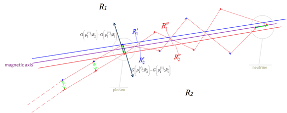
To understand the structure of a black hole we will look at what happens to a photon when it is captured by it the gravitational pull.

The model for light refraction that we introduced in earlier articles can be applied directly to photon moving through a black hole. Since we assume that the black hole is extremely massive, its trajectory will bring it towards the center of the black hole.

When moving along the magnetic axis of the black hole, the component $preon{{s}^{\left( + \right)}}$ of the $preo{{n}^{\left( + \right)}}$ pairs of the photon are pulled away from each other, splitting the photon into free $preon{{s}^{\left( + \right)}}$ which may or not recombine into neutrinos. This works as follow:

As we have seen earlier in this book, the force binding the $preon{{s}^{\left( + \right)}}$ of a $preo{{n}^{\left( + \right)}}$ pairs is gravitational. The QGD gravitational interaction between particles at the fundamental scale is $G\left( a;b \right)={{m}_{a}}{{m}_{b}}\left( k-\frac{{{d}^{2}}+d}{2} \right)$ , and since $a$ and $b$ are $preon{{s}^{\left( + \right)}}$ , ${{m}_{a}}={{m}_{b}}=1$ and since $d=1$ , the binding force between two $preon{{s}^{\left( + \right)}}$ of a $preo{{n}^{\left( + \right)}}$ pair is equal to $k-1$ .

For a photon moving along the magnetic axis, we have and $\displaystyle G\left( p_{1}^{\left\langle + \right\rangle };{{{{R}'}}_{2}} \right)-G\left( p_{1}^{\left\langle + \right\rangle };{{{{R}'}}_{1}} \right)>k-1$ where $\displaystyle p_{1}^{\left\langle + \right\rangle }$ and $\displaystyle p_{2}^{\left\langle + \right\rangle }$ are the component $preon{{s}^{\left( + \right)}}$ of a $preo{{n}^{\left( + \right)}}$ pair of a photon.

The regions ${{R}_{1}}$ and ${{R}_{2}}$ , on each side of the black hole axis are equally massive regions. If we call ${{{R}'}_{1}}$ and ${{{R}'}_{2}}$ the regions each side of $\displaystyle p_{1}^{\left\langle + \right\rangle }$ when the photon’s trajectory is aligned with the black hole axis then ${{{R}'}_{2}}>{{{R}'}_{1}}$ and $\displaystyle G\left( p_{1}^{\left\langle + \right\rangle };{{{{R}'}}_{2}} \right)-G\left( p_{1}^{\left\langle + \right\rangle };{{{{R}'}}_{1}} \right)>k-1$ . Similarly, if we call ${{{R}''}_{1}}$ and ${{{R}''}_{2}}$ the region on the each side $\displaystyle p_{2}^{\left\langle + \right\rangle }$ then ${{{R}''}_{1}}>{{{R}''}_{2}}$ and $\displaystyle G\left( p_{2}^{\left\langle + \right\rangle };{{{{R}''}}_{1}} \right)-G\left( p_{2}^{\left\langle + \right\rangle };{{{{R}''}}_{2}} \right)>k-1$ . So the force pulling the $preon{{s}^{\left( + \right)}}$ of $preo{{n}^{\left( + \right)}}$ pairs being greater than the force that binds them, the $preo{{n}^{\left( + \right)}}$ pairs are split into single $preon{{s}^{\left( + \right)}}$ .

How do we that the gravitational forces within a black hole are sufficiently strong to cause the photons to be broken down into $preon{{s}^{\left( + \right)}}$ ? If the gravitational forces within the black hole were not enough to breakdown the photons, then photons moving along a black hole axis would escape into space making the black hole visible. Since black holes do not emit light, then the gravitational interactions must be strong enough to break photons down into $preon{{s}^{\left( + \right)}}$ and neutrinos.

The image above shows how a simple two $preon{{s}^{\left( + \right)}}$ photon is split into two free $preon{{s}^{\left( + \right)}}$ which because of the the electro-gravitational interactions move back toward the magnetic axis. But, because the quantum-geometrical space occupied by the black holes is densely populated by particles which affect randomly the trajectories of the single $preon{{s}^{\left( + \right)}}$ , our two $preon{{s}^{\left( + \right)}}$ arrive at the magnetic axis of the black hole at different positions. And if they are in close enough proximity, the single $preon{{s}^{\left( + \right)}}$ will combine to form a neutrino which structure, not being made of $preon{{s}^{\left( + \right)}}$ pairs, remains structurally unaffected by the intense gravitational interactions within the black hole.

Once the trajectories of the $preon{{s}^{\left( + \right)}}$ or the neutrino coincides with the magnetic axis of the black hole, the $preon{{s}^{\left( + \right)}}$ or neutrinos will move through the center of the black hole and will exit it. $Preon{{s}^{\left( + \right)}}$ and neutrinos can escape the gravitation of the black hole because gravitational interactions, though it affects the directions of $preon{{s}^{\left( + \right)}}$ , doesn’t change their momentums which, as we have seen in earlier articles is fundamental and intrinsic (the momentum of a $preo{{n}^{\left( + \right)}}$ is $\left\| {\vec{c}} \right\|$ where $\vec{c}$ is momentum vector of a $preo{{n}^{\left( + \right)}}$ ).

It follows, that all matter that falls into a black hole will be similarly disintegrated into $preon{{s}^{\left( + \right)}}$ and neutrinos, which will exit the black hole. The black hole will thus radiate $preon{{s}^{\left( + \right)}}$ and neutrinos, in jets at both poles of their magnetic axis of rotation. Since $preon{{s}^{\left( + \right)}}$ and neutrinos interact too weakly with instruments to be detected by our instruments, they are invisible to them. In order to see the $preon{{s}^{\left( + \right)}}$ -neutrinos jets from a black hole, instruments may need detectors larger than our solar system. However, the jets can be observed indirectly when they interact with large amount of matter when the polarized $preon{{s}^{\left( + \right)}}$ and neutrinos they contain impart it with their intrinsic momentum. It is worth noting that polarized preons and neutrinos jets, as described by QGD, would contribute to the observed dark energy effect.

Based on QGD’s model of the black hole, we can predict that the $preon{{s}^{\left( + \right)}}$ /neutrino jets will form an extremely intense polarized $preon{{s}^{\left( + \right)}}$ field along the magnetic axis creating the equivalent of a repulsive electromagnetic effect at both poles. The polarized preonic field would repulse all matter on their path, which may explain the shape of galaxies.

From what we have discussed in the preceding section, we can define a black hole as an object which mass is such that it can breakdown all matter, including photons, into $preon{{s}^{\left( + \right)}}$ .

The QGD model of the physics of black hole has another important implication. The $preon{{s}^{\left( + \right)}}$ and neutrinos resulting from the breakdown of a particle or structure are indistinguishable from the $preon{{s}^{\left( + \right)}}$ or neutrinos resulting from the breakdown of any other particle or structure. This means, if QGD is correct, that all information about the original particle or structure is lost forever. That said, since this consistent from QGD’s axioms set and since, unlike quantum mechanics, QGD does not require that information be preserved, the loss of information it predicts does not lead to a paradox ( see this article for an excellent introduction to subject).

Cosmological Consequences

The mechanism of emission of $preon{{s}^{\left( + \right)}}$ and neutrinos will be continue until the black hole has been completely evaporated; which it will after it has absorbed all matter in its vicinity. By this mechanism, $preon{{s}^{\left( + \right)}}$ which had formed particles and structures are disintegrated into free $preon{{s}^{\left( + \right)}}$ and neutrinos which are then returned to the universe.

In later phases, the free $preon{{s}^{\left( + \right)}}$ and neutrinos will form new particles and structures, eventually leading to the formation cosmic structures and black holes. And later, due to gravitational interactions, these cosmic structures will ultimately be absorbed by black holes, which break down matter into $preon{{s}^{\left( + \right)}}$ and neutrinos, repeating the cycle indefinitely.

For a more complete discussion on the subject, see relevant sections in Introduction to Quantum-Geometry Dynamics.